About this tutorial
This tutorial turns Yann LeCun’s ~59-minute talk on world models into 15 modules you can study in order, with two runnable Python demos that were executed and verified while writing it. The talk argues that the next step in AI comes from systems that learn abstract, predictive models of the physical world (world models), plan by optimization, and are trained with joint-embedding (JEPA) rather than generative objectives.
Who it is for: engineers and researchers who know basic ML (neural nets, gradient descent, loss functions) and want the reasoning behind the talk, not just the slogans.
How to use it: read Modules 1–4 for the motivation, 5–7 for the architecture, 8–13 for the training machinery, and 14–15 for evidence and prescriptions. The section “Where this is contested” lists the positions other researchers hold, because several of LeCun’s claims are deliberately provocative.
Module 1 — The problem: Moravec’s paradox
Current machine learning learns far less efficiently than humans and animals, and it fails on exactly the tasks humans find trivial. That inversion is Moravec’s paradox, and it is the problem the whole talk sets out to solve.
The paradox in one table
| Easy for humans, hard for machines | Hard for humans, easy for machines |
| Clearing a dinner table, loading a dishwasher | Playing chess |
| Learning to drive in ~20 hours | Symbolic integration |
| Predicting that an unsupported object falls | Solving equations, proving theorems |
| Handling a task never seen before (zero-shot) | Recalling vast amounts of text |
The self-driving example. A teenager learns to drive in a few hours of practice. Autonomous-driving companies have millions of hours of driving data, yet imitation of that data has not produced level-5 autonomy. Consumer cars sit at level 2–3, and robotaxis rely on heavy engineering and extra sensors rather than learned understanding.
Why language misled the field. Language is discrete, low-dimensional and relatively clean. The physical world is continuous, high-dimensional and noisy. Techniques that work spectacularly on text (next-token prediction) do not transfer to sensory data, so progress on language says little about progress on the physical world.
The underlying claim: intelligence requires grounding in the physical world. LeCun acknowledges some philosophers and linguists disagree.
Check yourself: name one task in your own field that a 10-year-old could do zero-shot but no current system can do reliably. What would the system need to know about the world to do it?
Module 2 — Redefining intelligence
Intelligence is the ability to handle new situations quickly, not a stock of knowledge or skills. LeCun frames this with a line attributed to Jean Piaget: “Intelligence is not what you know, it’s what you do when you don’t know.” He notes the quote is apocryphal: psychologists distilled it from Piaget’s thinking.
What intelligence is not
- An accumulation of declarative knowledge. This is the main thing large language models (LLMs) provide, which is why LeCun treats them as useful but not intelligent in this sense.
- A collection of skills. With enough resources you can engineer a machine for almost any single task, including driving. That proves engineering effort, not intelligence.
What intelligence is: learning a new task with very few trials, or solving it zero-shot. Learning to drive in ~20 hours is the benchmark example.
Consequence 1: no simple measure. Any fixed benchmark can eventually be cracked by enough targeted effort. What matters is adaptation speed across tasks, which is hard to score.
Consequence 2: “AGI” is a misnomer. Human intelligence is specialized. People hold different knowledge and skills because they faced different environments. The defining trait is fast adaptation, not generality across everything. (LeCun’s company name reflects this: “Advanced Machine Intelligence” rather than AGI.)
Historical aside. In the 1975 Piaget–Chomsky debate on whether language is innate, Seymour Papert argued that simple learning machines like the perceptron were evidence that learning is possible. This is ironic: his 1969 book with Marvin Minsky, Perceptrons, had been blamed for stalling neural-network research for a decade.
Check yourself: why does LeCun argue that a high score on a fixed benchmark is weak evidence of intelligence?
Module 3 — Learning by observation
Infants learn most of their early world knowledge by watching, before they can act on the world, and machines can be tested for the same knowledge with the same method psychologists use on babies.
What is learned, roughly in order (approximate ages as stated in the talk):
| Age (approx.) | Concept acquired | How it is learned |
| ~2 months | A model of the infant’s own limbs; the world is 3-D | Motion parallax while being carried: depth is the best explanation for how the view changes as the head moves |
| Early months | Object permanence, stability, rigidity | Passive observation |
| ~9 months | Intuitive physics: gravity, inertia | Observation, then experiment |
The high-chair experiment. An 8–9-month-old will throw every toy off a high chair and watch it fall. The child is testing that gravity applies to everything, one object at a time.
Violation of expectation. Show an infant a toy car pushed off a platform that appears to float. A 6-month-old barely reacts; a 10-month-old stares, surprised. Surprise means the infant’s internal model predicted something else. Psychologists measure learned concepts this way.
Why this matters for machines: the same test works on AI. If a system has a predictive model of the world, its prediction error should spike on physically impossible events. Module 14 shows a self-supervised video model passing this test.
Check yourself: why is “the world is 3-D” learnable from passive video alone, with no labels?
Module 4 — The data argument, worked by hand
A four-year-old has taken in roughly as many bytes through vision as a frontier LLM sees in all its training text, about 10¹⁴ bytes each. LeCun uses this to argue that scaling text alone cannot reach human-level intelligence.
Step 1 — LLM training data
30 \times 10^{12}\ \text{tokens} \times 3\ \text{bytes/token} \approx 9 \times 10^{13} \approx 10^{14}\ \text{bytes}
The ~30 trillion tokens correspond to ~20 trillion words. At 250 words per minute, 8 hours a day, reading that takes about 457,000 years (the talk rounds to 400,000).
Step 2 — A child’s visual input
16{,}000\ \text{h} \times 3600\ \text{s/h} \times 2 \times 10^{6}\ \text{fibers} \times 1\ \text{byte/s} \approx 1.15 \times 10^{14}\ \text{bytes}
The 16,000 hours is waking time over four years, about 11 hours a day. The 2 million is the optic-nerve fiber count (both eyes), each carrying roughly one byte per second. (The transcript’s “16 hours” is a transcription error.)
Step 3 — Compare. Same order of magnitude. Text took humanity’s entire written output; vision took four years of one child. The same video volume is about 30 minutes of YouTube uploads.
The redundancy objection. “Video is far more redundant than text.” LeCun’s answer: redundancy is a feature. Self-supervised learning works by predicting one part of the data from another; with no redundancy there is nothing to predict and nothing to learn.
Verification: the arithmetic above was recomputed in Python while writing this tutorial (9.0 × 10¹³ vs 1.15 × 10¹⁴ bytes).
Check yourself: the 1 byte/s per fiber figure is an estimate. If it were 10× lower, does the argument still hold? What would it then imply about age?
Module 5 — Inference by optimization
An intelligent system should compute its answer by searching for the output that best satisfies an objective, not by a single fixed pass through a network. This search happens at inference time and is separate from learning.
Two modes of inference
| Feed-forward (reactive) | Inference by optimization | |
| How output is produced | Input passes through a fixed number of layers | Search over candidate outputs to minimize an objective |
| Compute per answer | Fixed | Variable: harder problems get more search |
| Example | An LLM producing one token | A planner choosing an action sequence |
| Psychology analogue | Kahneman’s System 1 (inferred) | System 2 deliberation (inferred) |
The energy function. The objective is a scalar function E(x, y) that is low when output y is compatible with input x and high otherwise. Inference means finding y that minimizes E given x:
\hat{y} = \arg\min_{y} E(x, y)
You can read E as a negative log-likelihood, but LeCun prefers the energy framing because it does not require normalized probabilities (Module 10).
Why LLM reasoning falls short of this. An LLM spends the same compute on every token. “Chain-of-thought” reasoning works by making the model emit more tokens to buy more compute. LeCun argues humans reason internally, in an abstract space, not in tokens or even in language.
Manual exercise. Let E(x, y) = (y² − x)². For x = 4, minimize by hand: E = 0 at y = 2 and y = −2. A feed-forward function must return one value; the energy view naturally represents both valid answers. This is why energy models suit problems with many correct outputs, such as predicting video.
Check yourself: for E(x, y) = (y² − x)², what does inference return for x = −1, and what does that tell you about the input?
Module 6 — The objective-driven architecture
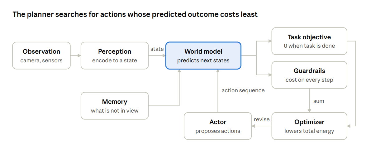
LeCun’s proposed agent perceives the world, imagines action sequences, uses a learned world model to predict their outcomes, and picks the sequence that minimizes a task cost plus guardrail costs. He laid this out in his 2022 position paper, A Path Towards Autonomous Machine Intelligence.
objective-driven agent · perceive, predict, score, optimize
The loop on the right runs at inference time: the actor proposes, the world model predicts, the costs score, and the optimizer revises until the energy is low.
The components
| Component | Role |
| Perception | Encodes the current observation into an abstract state representation |
| Memory | Supplies what is known but not currently perceived, completing the state estimate |
| Actor | Proposes candidate action sequences |
| World model | Predicts the next state from current state + action; applied repeatedly to predict a whole trajectory |
| Task objective | Scalar cost: 0 when the task is done, positive and growing with distance from done |
| Guardrail objectives | Costs that rise when a predicted state is unsafe; checked at every step of the trajectory |
The planning loop (model predictive control, MPC)
- Perceive: encode observation, combine with memory into state s₀.
- Propose an action sequence a₁ … aₖ.
- Roll the world model forward: s₁ = f(s₀, a₁), s₂ = f(s₁, a₂), …
- Score: total energy = task cost(sₖ) + Σ guardrail cost(sₜ).
- Optimize the actions to lower the energy (gradient descent or sampling).
- Execute the first action(s), observe again, re-plan.
This is classical MPC from 1960s optimal control. What is new is that the world model is learned from data and operates on learned representations.
The safety argument. LLM safety comes from fine-tuning, which can be jailbroken. In this architecture every output must minimize the guardrail objectives, so LeCun calls it “intrinsically safe”: there is no prompt that makes the optimizer ignore its own cost function. The argument assumes the guardrail costs are themselves correct (see “Where this is contested”).
Hands-on: a tested toy planner. The script below does the whole loop on a 2-D point mass that must reach a goal with a forbidden disc in the way. It learns the dynamics from random transitions (no equations given to the planner), then plans with the cross-entropy method, a sampling optimizer used in world-model planners such as DINO-WM.
import numpy as np

rng = np.random.default_rng(0)
DT, H = 0.1, 40
START, GOAL = np.array([0., 0.]), np.array([4., 0.])
WALL_C, WALL_R = np.array([2., 0.]), 0.8   # forbidden disc

def true_step(s, a):                    # s = [x, y, vx, vy], a = accel
    a = np.clip(a, -1, 1)
    p, v = s[:2], s[2:]
    v = 0.95 * v + DT * a               # friction the model must learn
    return np.concatenate([p + DT * v, v])

# 1. Observe random transitions
S, A_, S2 = [], [], []
for _ in range(200):
    s = np.concatenate([rng.uniform(-1, 5, 2), rng.normal(0, .5, 2)])
    for _ in range(10):
        a = rng.uniform(-1, 1, 2); s2 = true_step(s, a)
        S.append(s); A_.append(a); S2.append(s2); s = s2
X = np.hstack([np.array(S), np.array(A_)])

# 2. Learn the world model s' = A s + B a by least squares
W, *_ = np.linalg.lstsq(X, np.array(S2), rcond=None)
A_hat, B_hat = W[:4].T, W[4:].T
learned = lambda s, a: A_hat @ s + B_hat @ np.clip(a, -1, 1)

def rollout(model, s0, acts):
    s, traj = s0, []
    for a in acts:
        s = model(s, a); traj.append(s)
    return np.array(traj)

# 3. Energy = task cost + guardrail cost at EVERY step
def cost(traj, guard_w):
    task = np.sum((traj[-1, :2] - GOAL)**2) + 0.1*np.sum(traj[-1, 2:]**2)
    d = np.linalg.norm(traj[:, :2] - WALL_C, axis=1)
    guard = np.sum(np.maximum(0, WALL_R + 0.1 - d)**2)
    return task + guard_w * guard

# 4. Inference by optimization (cross-entropy method)
def plan(guard_w, iters=60, pop=400, elite=40):
    s0 = np.concatenate([START, [0, 0]])
    mu, sd = np.zeros((H, 2)), np.ones((H, 2))
    for _ in range(iters):
        cand = mu + sd * rng.standard_normal((pop, H, 2))
        costs = np.array([cost(rollout(learned, s0, c), guard_w) for c in cand])
        best = cand[np.argsort(costs)[:elite]]
        mu, sd = best.mean(0), best.std(0) + 1e-3
    return mu

# 5. Execute in the TRUE environment and test
def evaluate(acts):
    traj = rollout(true_step, np.concatenate([START, [0, 0]]), acts)
    return (np.linalg.norm(traj[-1, :2] - GOAL),
            np.linalg.norm(traj[:, :2] - WALL_C, axis=1).min())

for w, name in [(0.0, "no guardrail"), (1000.0, "with guardrail")]:
    g, m = evaluate(plan(w))
print(f"{name:15s} goal dist={g:.3f} min wall dist={m:.3f}")Test results (numpy 2.4, seed 0, run while writing this tutorial):
| Run | Final distance to goal | Closest approach to wall centre (radius 0.8) | Verdict |
| No guardrail | 0.047 | 0.032 | Drives straight through the forbidden disc |
| With guardrail | 0.035 | 0.902 | Reaches goal, stays outside the disc |
The learned model’s maximum error on training transitions was 3.6 × 10⁻¹⁵, as expected for linear dynamics. The full script also asserts these three conditions and printed ALL TESTS PASSED.
What the toy does not show: real world models predict in a learned representation space, not raw position and velocity, and real dynamics are nonlinear and stochastic. Modules 9–13 cover how that representation is learned.
Check yourself: set guard_w to 1.0 instead of 1000. Predict what happens, then run it. What does this tell you about the “intrinsic safety” claim?
Module 7 — Hierarchical planning
Real plans must be built at several levels of abstraction at once, and nobody yet knows how to learn this; LeCun calls it a completely open problem and an ideal PhD topic.
Why flat planning fails. Planning a trip from an NYU office to Paris in 10-millisecond muscle commands is impossible for two reasons: the sequence is far too long, and the information does not exist yet (you cannot know how long you will wait for a taxi).
The decomposition LeCun walks through
- Be in Paris tomorrow
- Get to the airport (~1–1.5 h, details unknown)
- Get down to the street
- Walk to the elevator, press the button, ride down, walk out
- Stand up from the chair (a learned reflex, no deliberate planning)
- Walk to the elevator, press the button, ride down, walk out
- Hail a taxi, ride to the airport
- Get down to the street
- Catch the plane
- Get to the airport (~1–1.5 h, details unknown)
Each level sets a subgoal for the level below. Upper levels use coarse predictions (“about an hour to the airport”) with few details. Near the bottom, actions become familiar enough to run as a policy: a direct mapping from state to action with no search.
What a hierarchical world model needs (the open questions):
- Representations at multiple abstraction levels, learned rather than hand-designed.
- World models at each level that predict over different time scales.
- A way for a high-level plan to hand subgoals down as objectives for the level below.
- A way to decide when a sub-task is familiar enough to switch from planning to a policy.
Check yourself: in the trip example, which level would a sudden flight cancellation force to re-plan, and which levels could stay unchanged?
Module 8 — Why generative models fail at video prediction
Predicting the future pixel by pixel forces a model to spend its capacity on details that are fundamentally unpredictable, so it learns poor representations; LeCun says he lost about ten years to this approach.
How self-supervised learning works on text. Corrupt the input (mask some words), train a network to reconstruct the missing parts. BERT masks words anywhere; an LLM is the special case that masks only the last word. This works and scales because the vocabulary is finite: the model can output a probability for every possible token.
Why the same recipe breaks on video
| Text | Video | |
| Possible next items | ~100,000 tokens | Effectively infinite frames |
| Can you output a full distribution? | Yes, a softmax over tokens | No tractable way |
| What a regression model predicts | n/a | The average of all futures: a blur |
The auditorium example. Pan a camera across a lecture hall and stop. A model can reasonably predict that the room continues, has a finite size, maybe windows. It cannot predict each audience member’s face or which seats are empty. Training it to predict those pixels penalizes it for information it could never have.
The blurry-prediction result. A ~2015 experiment predicted 2 future frames from 4 context frames and produced blurry outputs: the network averaged over all plausible futures. GANs, and later latent-variable models such as diffusion, fix the blur.
“But video generators make convincing videos.” LeCun’s answer has two parts:
- Good video generators mostly predict in a representation (latent) space first; a second stage renders pixels.
- A generator only needs to produce one plausible video. A world model needs to represent the space of all plausible futures to plan. Producing a sample is a much easier problem, and evidence that generators understand physics is weak.
Check yourself: why is predicting the average future the optimal answer for a model trained with squared error, and why is that average useless for planning?
Module 9 — JEPA: Joint Embedding Predictive Architecture
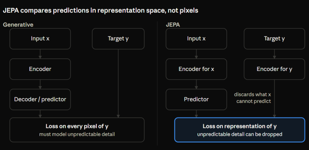
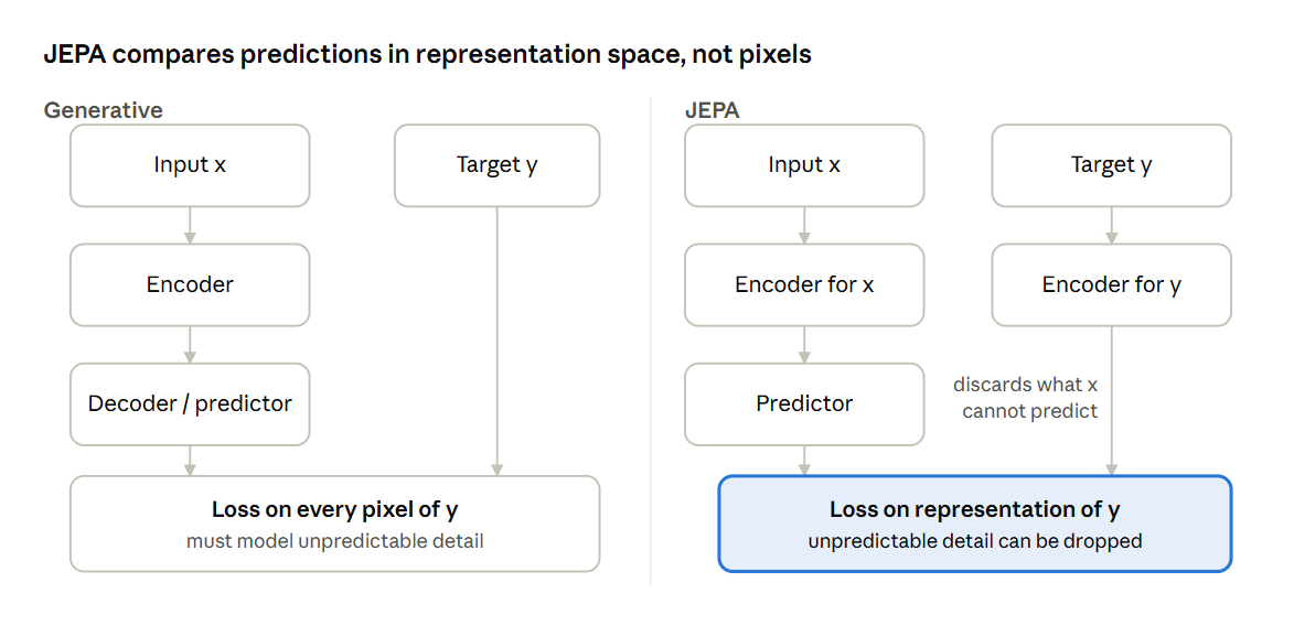
JEPA encodes both the observed input and the target, then predicts the target’s representation rather than its raw content, which lets the encoder discard everything unpredictable.
generative vs joint-embedding predictive architecture
The only structural change is a second encoder on y; it moves the loss from pixels to representations, which is what lets JEPA ignore unpredictable detail.
Side by side
| Generative architecture | JEPA | |
| Inputs | Observation x (and action a) | Observation x, target y (and action a) |
| Encoders | x only | x and y, each into a representation |
| What is predicted | y itself, in full detail (pixels) | The representation of y |
| Loss | Reconstruction error in input space | Prediction error in representation space |
| Unpredictable detail | Must still be modelled | Can be dropped by the y-encoder |
| Main failure mode | Blur / wasted capacity | Collapse (Module 10) |
Why predicting in representation space helps. The y-encoder is free to throw away details that x gives no evidence about: the faces in the auditorium, leaf positions in wind. Predictions become more abstract, with fewer details, but more accurate on what remains.
Evidence LeCun cites: across self-supervised image and video methods, the best-performing representations come from joint-embedding methods, not reconstruction. When features from reconstruction-trained models (e.g. masked autoencoders, MAE) are fed to a supervised downstream head, results are weaker. About 1,700 papers on Google Scholar mention the spelled-out phrase “joint embedding predictive architecture” (as stated in the talk).
Two ways to build the training pair
- Two views: two transformations of the same scene; train their representations to agree.
- Corruption: mask or transform the input; predict the representation of the original from the representation of the corrupted version. I-JEPA and V-JEPA use masking.
The catch. If the only goal is low prediction error, the encoders can output a constant for every input. Prediction then becomes trivially perfect and nothing is learned. Preventing this collapse is the central design problem of joint-embedding learning.
Check yourself: an autoencoder with an unrestricted code can also “collapse”. What is the autoencoder’s trivial solution, and how is it different from JEPA’s?
Module 10 — Collapse, energy-based models, and how to prevent it
Every joint-embedding method is defined by its anti-collapse mechanism; LeCun groups them into contrastive and regularized families and prefers regularized methods that maximize information across representation dimensions.
Energy-based models (EBMs) in one picture. Data points (x, y) sit in valleys of an energy landscape E(x, y); away from the data the energy rises like altitude around a lake. Given x, inference returns the y values in the valley, and there can be several (Module 5). Given y, you can infer x the same way. Probabilistic models are the special case where E has a normalized form and is trained with likelihood.
Collapse in EBM terms: a flat landscape, low everywhere. An autoencoder that learns the identity, or a JEPA that ignores its input, both produce it.
Two families of fixes
| Family | Mechanism | Trade-off |
| Contrastive | Generate points away from the data and push their energy up | Needs many good negatives; becomes inefficient in high dimension |
| Regularized | Limit the volume of space that can have low energy, so pushing data down forces everything else up | Needs a good, differentiable regularizer |
Information maximization, made concrete. Run a batch through the encoder to get a matrix: one row per sample, one column per representation variable.
- Sample-contrastive: make the rows different from each other. CLIP (image–text joint embedding, used in many LLM vision front-ends), SimCLR and MoCo are examples.
- Dimension-contrastive: make the columns different and decorrelated, so each variable carries independent information. VICReg, Barlow Twins, MCR² and MMCR are examples. LeCun prefers this family.
The measurement problem. Maximizing information needs a differentiable measure of it. Two obstacles:
- Proper information measures require the distribution; we only have a finite batch of samples.
- Maximizing should push on a lower bound, but practical estimates are upper bounds. In practice: pick a good upper bound, prove what you can, and verify empirically.
Manual exercise. Write a 4 × 3 batch matrix where every row is identical. Which family’s loss is violated? Now write one where column 2 always equals column 1. Which family catches that, and which misses it?
Module 11 — Abstraction: what a world model should be
A world model should predict in an abstract space that ignores detail, the way science does; it should not be a pixel simulator, a “digital twin”, or a video generator.
Science already works this way. You could in principle simulate this room at the level of quantum field theory, but it is useless for predicting whether the audience is bored. Science stacks abstractions, each ignoring the details below it to make longer-range predictions possible:
quantum fields → particles → atoms → molecules → proteins → cells → organs → organisms → individuals → societies → ecosystems
Each level also holds knowledge not obviously derivable from the level below: chemistry is not just applied physics in practice.
The airfoil example. Computational fluid dynamics models air as velocity and density in small cells and solves the Navier–Stokes equations. The real mechanism is molecules colliding, but simulating those would be intractable and would diverge from reality faster because of the extra detail. Accurate long-range prediction requires dropping detail.
When you need a learned world model. A robot’s own body can be written as equations, which is why humanoids can do scripted acrobatics. Once a system interacts with a messy environment (a robot handling objects, a jet engine, a chemical plant, a patient), you cannot write the equations. You need a learned, phenomenological model of the system plus its environment, good enough to plan actions.
LeCun’s three “do not” rules for world models
- Do not build simulators of every detail (“digital twins”).
- Do not build generative models of the observations.
- Do not confuse video generation with world modelling: if you want cute videos, build a generator; if you want to control robots or processes, do not.
Check yourself: pick a system you work with. What are its “molecules” (details you could log but never need) and its “fluid variables” (the abstraction you actually reason with)?
Module 12 — SIGReg, step by step
SIGReg (Sketched Isotropic Gaussian Regularization) prevents collapse by pushing the batch of embeddings toward an isotropic Gaussian, checked one random 1-D projection at a time; it is LeCun’s preferred method, simple enough to train on one GPU, and not yet scaled up.
Why an isotropic Gaussian? In an isotropic Gaussian every variable is independent of the others, with equal variance. Independent variables are individually maximally informative, which is exactly the dimension-contrastive goal from Module 10. (It is also the maximum-entropy distribution for a given variance, which LeCun mentions but sets aside.)
The problem it solves. You have a few hundred to a few thousand points in, say, 2,000 dimensions, and no density. How do you test “is this Gaussian” and get a gradient?
The trick, in four steps
- Pick a random unit direction u and project every embedding onto it. You now have N numbers: a 1-D marginal.
- Compare their empirical distribution (a staircase CDF) with the standard Gaussian CDF.
- For each point, the comparison says whether it sits too far left or right: that is its gradient.
- Repeat for many directions and sum. Backpropagate through the encoder so the points move.
The guarantee comes from the Cramér–Wold theorem: a multivariate distribution is fully determined by all its 1-D projections. If every projection is Gaussian, the joint distribution is Gaussian.
Manual walkthrough (one projection, N = 4). Projected values: 0, 0.1, 0.2, 3.0. The Gaussian quantiles at ranks (i + 0.5)/4 are −1.150, −0.319, 0.319, 1.150.
| Rank | Projected value | Target quantile | Difference | Gradient step moves the point |
| 1 | 0.0 | −1.150 | +1.150 | Left |
| 2 | 0.1 | −0.319 | +0.419 | Left |
| 3 | 0.2 | +0.319 | −0.119 | Right |
| 4 | 3.0 | +1.150 | +1.850 | Left (strongly) |
Loss = mean of squared differences = (1.323 + 0.176 + 0.014 + 3.423) / 4 ≈ 1.234. The cluster spreads out and the outlier is pulled in. Matching sorted values to quantiles like this is one way to compare the staircase with the Gaussian; the LeJEPA paper uses a different 1-D test (Epps–Pulley, on characteristic functions), but the principle is identical.
Now automate it (numpy, tested). Demo A reproduces the talk’s “X” picture by moving points directly. Demo B trains a linear encoder on two noisy views of the same data, with and without SIGReg, to show collapse and its prevention.
import numpy as np
from scipy.stats import norm

rng = np.random.default_rng(0)

def sigreg(Z, n_dirs=256):
    """Return (loss, dL/dZ) for embeddings Z of shape (N, D)."""
    N, D = Z.shape
    U = rng.standard_normal((D, n_dirs))
    U /= np.linalg.norm(U, axis=0)                 # random unit directions
    P = Z @ U                                      # 1-D projections
    order = np.argsort(P, axis=0)
    q = norm.ppf((np.arange(N) + 0.5) / N)         # Gaussian quantiles
    target = np.empty_like(P)
    np.put_along_axis(target, order, q[:, None].repeat(n_dirs, 1), axis=0)
    diff = P - target                              # each point vs its rank's quantile
    loss = np.mean(diff ** 2)
    dP = 2 * diff / (N * n_dirs)
    return loss, dP @ U.T

def stats(Z):
    C = np.cov(Z.T)
    corr = C / np.sqrt(np.outer(np.diag(C), np.diag(C)))
    off = np.abs(corr[~np.eye(len(C), dtype=bool)]).max()
    u = rng.standard_normal((Z.shape[1], 500)); u /= np.linalg.norm(u, axis=0)
    p = (Z - Z.mean(0)) @ u
    kurt = np.mean(p**4, 0) / np.mean(p**2, 0)**2 - 3   # 0 for a Gaussian
    return np.sqrt(np.diag(C)).round(2), off, np.abs(kurt).mean()

# Demo A: Gaussianize an "X" by moving the points
def demo_a(N=2000, D=16, steps=400, lr=20.0):
    t = rng.uniform(-3, 3, N); arm = rng.integers(0, 2, N)
    Z = np.zeros((N, D))
    Z[:, 0] = t
    Z[:, 1] = np.where(arm == 0, t, -t)            # an "X" in dims 0-1
    Z[:, 2:] = 0.05 * rng.standard_normal((N, D - 2))
    before = stats(Z)
    for _ in range(steps):
        _, g = sigreg(Z)
        Z -= lr * N * g / 10
    return before, stats(Z)

# Demo B: collapse with vs without SIGReg
def demo_b(lam, N=1024, Din=32, D=8, steps=1500, lr=0.5):
    latent = rng.standard_normal((N, D))
    X = latent @ rng.standard_normal((D, Din))     # data with 8 real factors
    W = 0.1 * rng.standard_normal((Din, D))        # linear encoder
    for _ in range(steps):
        x1 = X + 0.3 * rng.standard_normal(X.shape)   # two noisy views
        x2 = X + 0.3 * rng.standard_normal(X.shape)
        z1, z2 = x1 @ W, x2 @ W
        g_inv = 2 * (z1 - z2) / N                  # invariance loss gradient
        gW = x1.T @ g_inv - x2.T @ g_inv
        if lam > 0:
            _, g_reg = sigreg(z1, n_dirs=64)
            gW += lam * x1.T @ g_reg
        W -= lr * gW / Din
    Z = X @ W
    rank = np.sum(np.linalg.svd(Z - Z.mean(0), compute_uv=False) > 1e-3 * np.sqrt(N))
return Z.std(0).mean(), rankTest results (numpy 2.4, scipy 1.17, seed 0, run while writing this tutorial):
| Run | Std of first 4 dims | Max abs correlation | Mean abs excess kurtosis | Effective rank |
| A: “X” before | 1.74, 1.74, 0.05, 0.05 | 0.07 | 0.58 | n/a |
| A: after SIGReg | 1.00, 1.00, 1.00, 1.00 | 0.00 | 0.07 | n/a |
| B: invariance loss only | mean 0.0003 | n/a | n/a | 0 of 8 (collapsed) |
| B: invariance + SIGReg | mean 0.94 | n/a | n/a | 8 of 8 |
The script asserts all four outcomes and printed ALL TESTS PASSED. One debugging note: at a learning rate of 0.05, the invariance-only run had only shrunk to 0.54 after 1,500 steps. Collapse is gradual, so a short training run can hide it.
The lesson hidden in row A-before. The “X” already has near-zero linear correlation (0.07) because its two arms cancel out, yet dims 0 and 1 are strongly dependent. A covariance-based regularizer would see nothing wrong. The excess kurtosis exposes it, and SIGReg removes it, because matching full 1-D distributions captures more than second-order statistics.
The theory result mentioned in the talk. A recent paper shows that if the true explanatory variables are Gaussian and observations are a nonlinear warp of them (a spiral, say), an encoder trained with SIGReg recovers the original variables up to a rotation. It is a special-case guarantee, not a general proof.
Check yourself: why does Demo B collapse when the only loss is “make the two views’ embeddings match”? Write the trivial solution for W.
Module 13 — Distillation methods: the ones that already scale
Distillation methods prevent collapse without an explicit information term, by making the target encoder a slow-moving average of the online encoder; they are less principled than SIGReg in LeCun’s view, but they are the methods already scaled to strong image and video results.
The architecture
- Two encoders with the same architecture: an online (student) encoder and a target (teacher) encoder.
- The input is masked, cropped or corrupted for the online branch; the target branch sees the full or a different view.
- A predictor maps the online representation to the target representation.
- Gradients flow only through the online encoder and predictor. The target branch has a stop-gradient.
- The target encoder’s weights are an exponential moving average (EMA) of the online weights:
\theta_{\text{target}} \leftarrow \tau \, \theta_{\text{target}} + (1 – \tau) \, \theta_{\text{online}}, \qquad \tau \approx 0.99\text{–0.999}
The target lags behind, so the online encoder chases a slowly moving goal instead of a constant it could trivially match. Why this avoids collapse is still not fully explained theoretically, which is why LeCun calls it intuition-driven.
Lineage of the methods named in the talk
| Method | Origin | What it showed |
| BYOL (“Bootstrap Your Own Latent”) | Google DeepMind | EMA target, borrowed from variance-stabilizing tricks in reinforcement learning, works for self-supervised images |
| MoCo and successors | Meta | Momentum (EMA) encoders at scale |
| I-JEPA | Meta | Masked image prediction in representation space; better and much faster to train than the generative MAE |
| DINO (v2, v3) | Meta, Paris | Joint embedding + distillation with heavy engineering; today’s best general-purpose image encoder per the talk |
| V-JEPA (2, 2.1) | Meta | Masked video prediction in representation space; state of the art on action recognition and anticipation |
Practical takeaway from the talk: if you need an image encoder for a vision task today, DINO is the default choice. Several robot demos at the event used it.
Check yourself: what would happen if τ were set to 0, so the target equals the online encoder at every step?
Module 14 — The evidence
LeCun offers three kinds of evidence that self-supervised joint-embedding models learn real world structure: they support planning, they show surprise at impossible events, and their features encode 3-D depth without being trained for it.
1. Planning with a learned world model. A DINO encoder plus a trained world model drives a planner that reaches goal configurations in simulated environments with complex dynamics, in under 25 steps (this matches the published DINO-WM work; the talk does not name it). Tasks mentioned: double pendulum and “push-T”. SIGReg-trained action-conditioned world models also plan simple robot tasks in simulation. Module 6’s toy planner is the same loop at miniature scale.
2. Violation of expectation (machine common sense). V-JEPA is trained to predict the representation of upcoming video. Slide a 16-frame window along a test video and log the internal prediction error at each step. When something physically impossible happens, such as a thrown ball vanishing, the error spikes. This is the infant test from Module 3, applied to a network. LeCun calls it the first time he has seen a fully self-supervised system acquire some common sense.
How to run this test yourself (procedure):
- Take a trained video predictor with an encoder and a predictor.
- Prepare matched pairs of clips: one physically possible, one with a single violation (object vanishes, passes through a wall, floats).
- For each time step, compute the distance between predicted and actual next-window representations.
- Compare the error curves: a model with intuitive physics shows a spike only at the violation in the impossible clip.
3. Depth from a single image. Freeze V-JEPA 2.1’s encoder, train a small head on top to predict depth from one image. The talk reports results better than a strong baseline (“the V3” in the transcript, probably DINOv3). The model was never trained on depth; it learned that the world is 3-D from predicting video, as infants do. The same features also segment objects decently.
Check yourself: why does training only a small head on a frozen encoder count as evidence about the encoder, rather than about the head?
Module 15 — LeCun’s prescriptions and the Q&A
LeCun closes with five recommendations for anyone working on AI for the physical world, which he admits make him unpopular in Silicon Valley.
| Abandon (or minimize) | In favour of | His reason |
| Generative models | Joint-embedding architectures (JEPA) | Unpredictable detail wastes capacity (Modules 8–9) |
| Probabilistic models | Energy-based models | More general; no normalization needed (Modules 5, 10) |
| Contrastive methods | Regularized, information-maximizing methods | Scale better with dimension (Module 10) |
| Reinforcement learning | Model-predictive control on learned world models; RL only on top of good representations | RL is extremely sample-inefficient: “what you do when you’re desperate” |
| Working on LLMs (in academia) | Grounded / physical AI | Academia cannot compete at LLM scale, and LLMs cannot handle high-dimensional, continuous, noisy data |
Where this is going. LeCun left Meta at the end of the previous year and founded AMI Labs, targeting “AI for the real world”: robotics, but also industrial process control and any high-dimensional, continuous, noisy problem where LLMs are, in his words, completely helpless.
The Q&A: how do you put engineering constraints into a learned representation space? An engineer asked how to express “don’t hit the wall” when the world model works on abstract embeddings rather than 3-D coordinates.
Answer: train a very small head (essentially a projection) on top of the frozen representation that maps it to the quantity you care about. Each constraint or task objective gets its own small head. Because the representation already carries the structure, a head like “is the door open?” needs very few labelled samples. Module 6’s toy sidesteps this by planning in raw coordinates; a real system would replace cost() with such learned heads.
Check yourself: a learned guardrail head can be wrong. How would you test one before trusting the planner that optimizes against it?
Where this is contested
The talk is an advocacy piece by one of the field’s most prominent researchers, and several of its claims are actively disputed; treat the table below as the counter-case, drawn from general knowledge of the debate rather than from sources looked up for this tutorial.
| LeCun’s claim | Counter-position held by other researchers | Status |
| Scaling LLMs cannot reach human-level intelligence | LLMs plus multimodal training and RL-based reasoning keep improving; probing studies (e.g. Othello-GPT) suggest LLMs build internal world models from text | Open, heavily debated |
| Video generators are not world models | Several labs explicitly frame video generators as world simulators (e.g. Genie, Cosmos) and use them for agent training | Open; benchmarks show generators often break physics |
| The 10¹⁴-byte comparison shows text is insufficient | Raw sensory bytes overstate information content; text is highly compressed knowledge, so equal byte counts do not mean equal information | The arithmetic is right; the interpretation is disputed |
| Minimize reinforcement learning | RL drove major results in games, robotics and LLM reasoning post-training | LeCun agrees RL is useful on top of good representations; disagreement is about how much |
| Guardrail objectives make the system “intrinsically safe” | An optimizer will exploit errors in a learned world model or a misspecified cost; this is a known failure in model-based RL | The architecture removes prompt jailbreaks, not specification errors |
| SIGReg is the preferred anti-collapse method | Distillation methods (DINO, I-JEPA) are what currently work at scale | LeCun himself says SIGReg still needs scaling |
Open questions LeCun himself names: hierarchical planning (Module 7), scaling SIGReg, and how to measure information content with a proper lower bound (Module 10).
How to read the talk well: separate the engineering content (JEPA, collapse prevention, MPC planning), which is well grounded and reproducible, from the strategic forecasts (what will or will not reach human-level AI), which are judgments under uncertainty.
Answers to the self-checks, and glossary
Short answers to each module’s “Check yourself” question; try them first.
| Module | Answer |
| 1 | Open-ended. Typical answers involve physical manipulation or novel situations; the missing piece is usually a predictive model of how objects behave. |
| 2 | Any fixed benchmark can be cracked with enough targeted engineering, so a score measures effort spent on that task, not adaptation speed. |
| 3 | Depth is the simplest explanation for how the image changes as the viewpoint moves (parallax), so a predictor of the next view must represent it. |
| 4 | At 0.1 byte/s the child total is ~10¹³, matched only after ~35 years of waking hours rather than 4; the conclusion weakens but sensory data still rivals all text within a human lifetime. |
| 5 | No real y satisfies y² = −1; the minimum is y = 0 with E = 1. The non-zero energy signals the input has no compatible answer. |
| 6 | Measured: at weight 1.0 the plan still stayed safe (closest approach 0.893) because detouring was cheap. A soft guardrail is only as strong as its weight relative to task pressure; under a tighter time budget it could be traded away. Hard constraints are safer. |
| 7 | The high level (“catch the plane”) re-plans; low-level skills such as walking stay unchanged. |
| 8 | Squared error is minimized by the conditional mean; the mean of many sharp futures is a blurry frame that matches none of them, so no plan can use it. |
| 9 | The autoencoder’s trivial solution is the identity (copy input to output); JEPA’s is a constant output that ignores the input. |
| 10 | Identical rows violate sample-contrastive losses. A duplicated column is caught by dimension-contrastive losses; sample-contrastive losses can miss it. |
| 11 | Open-ended. |
| 12 | Invariance alone is minimized by W = 0: every input maps to the same point, so the views always match. |
| 13 | With τ = 0 the target is the online encoder with a stop-gradient, removing the lag; collapse becomes much more likely. |
| 14 | A small head trained on a frozen encoder cannot create depth knowledge from little data; the information must already be in the features. |
| 15 | Test it on held-out labelled states, especially near the boundary, and adversarially: let the planner search for states the head scores as safe, then check them in reality or simulation. |
Glossary
| Term | Meaning |
| World model | A learned predictor of the next state of the world given the current state and an action |
| JEPA | Joint Embedding Predictive Architecture: predict the representation of the target, not the target itself |
| Energy function | A scalar score of compatibility between variables; low = compatible |
| Collapse | Encoders producing constant or low-information outputs that trivially minimize the training loss |
| Contrastive method | Prevents collapse by pushing up energy on generated negative samples |
| Regularized method | Prevents collapse by limiting the volume of low-energy space |
| SIGReg | Sketched Isotropic Gaussian Regularization: Gaussianize embeddings via random 1-D projections |
| EMA target encoder | A teacher whose weights are a slow moving average of the student’s |
| MPC | Model predictive control: optimize an action sequence through a model, execute, re-plan |
| Moravec’s paradox | What is easy for humans (perception, motion) is hard for machines, and vice versa |
| Violation of expectation | Measuring learned knowledge through surprise at impossible events |